|
Home DH-Debate 5. Pleistocene 7. Holocene |
| 1. Introduction | 2. Lakes in late Pleistocene |
| 3. Floods in late Pleistocene | 4. Literature |
Last glacial absolute maximum took place about 26,500 to 19,000 years ago. The ice sheet covered then the whole of Scandinavia and the Baltic region down to North
Poland and Germany. In North America, the ice cap extended down to the Great Lakes between Canada and the United States.
|
|
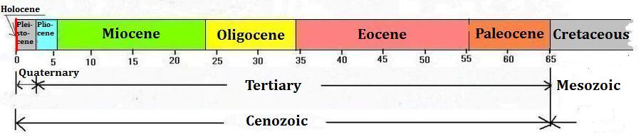
Cenozoic is the period of mammals, which followed the Mesozoic which was
the period of the dinosaurs. Tertiary is that part of Cenozoic where no
humans existed, and Quaternary represents the part of Cenozoic when there were
humans. Quaternary is subdivided into Pleistocene and Holocene. Holocene represents the present which basically is a Pleistocene interglacial period. The climate in the last phases of the Pleistocene is the subject of this article.
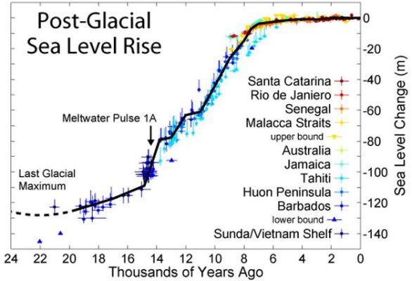
Drill cores from the inland ice show that the temperature in the Antarctic began to increase about 17,000 years ago, causing sea surface level to rise.
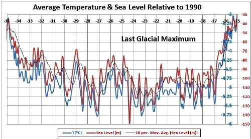
Average temperature and sea surface level from 35,000 to 15,000 years before present related to the present level (1990) by L. David Roper. The blue line
represents the temperature and the red represents sea surface level. The thin black line shows the sea surface level smoothed with a 10 period rolling mathematical average. Time progresses from left to right. It is seen that the World's Sea surface level during "Last Glacial Maximum" was more than 100 meters below today. The figure also shows that a rise in sea surface level - and thus a temperature increase - began rather abruptly about 17,000 years before present.
During the next close to 9,000 years the ice cap in Scandinavia dwindled slowly and became the smaller glaciers in the Norwegian mountains that we know today.
The warming happened quite irregular, Uriarte writes. In some periods the sea surface level of the World's oceans could rise 10 meters or more during a few hundred years. Such a sudden increase coincided with Bølling-Allerød warm period about 14,000 years ago, when sea levels rose by 20 meters. Another warm period occurred 11,000 years ago at the start of the Holocene. Some have calculated that during warm periods sea surface level increased by up to 50 mm. per year, while it varied by only about 3 mm. per year in between warm periods.
|
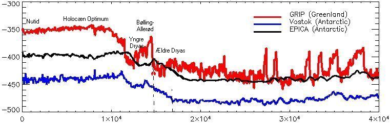
Oxygen isotope ratio through 40,000 years found in ice cores from Greenland and
Antarctica. The relationship between heavy and light oxygen isotopes indicates
temperature. It looks like the warming began 17,000 years ago in Antarctica. In the northern hemisphere, the warming in earnest began only 15,000 years ago with the Bølling-Allerød warm period. This is not consistent with the expectations that one may have following the Milankovitch theory, according to which the northern hemisphere is assumed to be climatically governing. On Antarctica, it has generally been pretty cold all the time, while the northern hemisphere has experienced several temporary warm and cold periods. Also, note the characteristic shape of the warm periods, the heat comes suddenly, probably within a few decades, and then it fades slowly away. Temperature graphs for actual interglacial periods typically also have this shape.
The warming did not occur at the same time across the globe. The temperature increase happened first in the southern hemisphere. Only with the beginning of the Bølling-Allerød heating period about 14,000 years ago, the temperature rose significantly in the northern hemisphere. This warming period was largely confined to the northern part of the planet. Analyses of sediments from the seabed off the mouth of the Murray River in Australia show no indication of the Bølling-Allerød warming period and also no evidence of the subsequent Younger Dryas cold period.
|
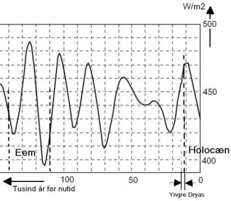
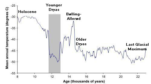
Top: The theoretical Milankovitch insolation at 65 degrees north latitude during the last 100,000 years calculated by Berger. It is seen that the insolation was quite high in the cold Younger Dryas period. We also note that the present insolation is pretty low. Time progresses from left to right.
Bottom: The temperature on the surface of the Greenland ice sheet during the "Last Glacial Maximum" (LGM), Older Dryas, Bølling-Allerød and Younger Dryas. Time progresses from right to left.
It is commonly believed - by some - that the reason for the completion of the Weichsel glaciation shall be sought in an increased Milankovitch insolation (solar radiation) in the northern hemisphere. Some 17,000 years before present the theoretical July insolation on 65 degrees north latitude was 430 W/m2, then it increased to a maximum of more than 470 wat/m2 about 10,000 years before present. In present times, the theoretical insolation at 65 degrees north latitude is fairly low that is back to around 430 W/m2 (calculated by Berger).
Reindeer hunters, who belonged to the Hamburg culture lived in Northern Europe at the end of the Weichel glaciation. Many believe that they were descendants of the Cro Magnon ice age hunters.
The last phase of the actual ice age around 16-17,000 years before present is called Older Dryas. It was a very cold period. Dryas is the Latin name for the
hardy arctic herb, in the family with mountain avens, which is characteristic of very cold Arctic landscapes.
For almost 15,000 years ago started a marked warming that has been named the Bølling-Allerød warm period after the Bølling Lake and Allerød clay pit, which are the sites in Denmark, where it was first observed. The climate in this warm period was cool but warmer than the ice age. Organic deposits found in Allerød showed that the vegetation was dominated by mountain avens, birch, sea buckthorn, crowberry and arctic willows - not unlike the vegetation on Svalbard today. The reindeer was the dominant large animals, perhaps hunted by predators like wolverine and lynx.
Some estimates based on pollen analysis and other organic traces show that
average July temperature was about 11 degrees that should be compared
with the around 18 degrees, which is the average July temperature in today's
Denmark. A July temperature of about 11 degrees will correspond to the current climate in northern Scandinavia or Canada. Analyses of the Greenland ice cores show that the temperature during the period was far from stable, there were several significant cold spells.
|
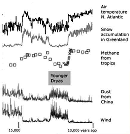
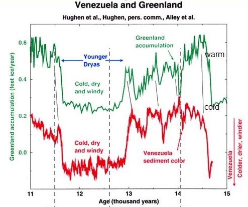
Left: The climate of the Younger Dryas as reflected by dust in the cores from
Greenland - Windblown dust from China testifies that the cold and thus dry climate of the Younger Dryas prevailed at least in the northern hemisphere and it thus was not an isolated North Atlantic phenomenon. This makes the Lake Agassiz - Gulf Stream theory less likely. By Alley et al, PNAS 2000.
Right: The growth of the Greenland ice sheet compared with analysis of
sediments at the bottom of the lake in Venezuela. As you can see the cold period of Younger Dryas also left its traces in Venezuela.
But however, about 13,000 years before present the Bølling-Allerød warm period came to a completion, and the arctic temperatures returned with the cold
Younger Dryas period. The climate of this period was not quite as harsh as the Older Dryas. It has been estimated from pollen analysis and similar that the average July temperature in southern Scandinavia was around 8-9 degrees, rising throughout the period. This is roughly equivalent to today's July average temperature in Alaska and Siberia.
Younger Dryas can be traced many places in the northern hemisphere, both as
an increase in the quantity of dust from China in the Greenland ice sheet and as
a color change in sediments of a lake in Venezuela.
In spite of energetic search is not, however, found solid evidence of Yuonger Dryas on the Southern Hemisphere. For example, analyzes of sediments in the seabed off the mouth of the Murray River in Australia show no trace of a Younger Dryas cold spell.
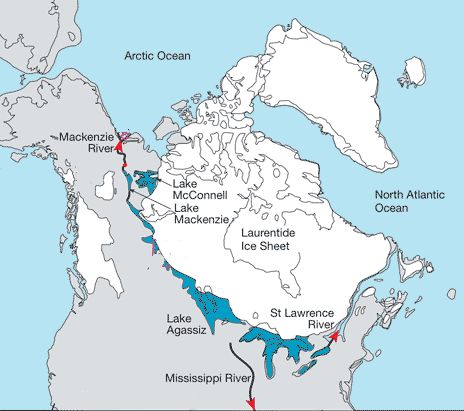
By the melting of the North American inland ice huge ice lakes of melt-water formed along the edge of the glacier, including Lake Agassiz. The Ice lakes had all connection with each other, and it is assumed that there were three drainages to the world Sea: the Mackenzie River, St. Lawrence River and the Mississippi. It is seen that the Great Lakes between the United States and Canada has their origin from the end of Ice Age like so many others lakes.
There have been many speculations about the possible causes of the end of the Bølling-Allerød warm period and the return of the cold climate in the area around the North Atlantic. Milankovitch's theory can not help us, according to this theory the July-insolation at 65 degrees northern latitude at this time was about 450 W/m2 and increasing, which is much higher than today, where the theoretical insolation at the same latitude is about 430 W/m2.
The prevailing theory is that a huge meltwater lake called Lake Agassiz,
containing more ice cold fresh water than all of today's lakes together, it is said, discharged all its water into the North Atlantic. Initially, the lake was cut off from the world Sea by parts of the glacier, but suddenly the ice dam broke and the entire lake's content of ice-cold fresh water was discharged into the North Atlantic. Thus the sea-water became less salt and froze easier in the winter, the sea ice covered a larger area and disturbed thereby the Gulf Stream, creating a cold spell in Northern Europe and America that lasted about 1,500 years.
The Gulf Stream is likely to exist based on objective geographical and climatic conditions, and one can argue that if it only returned to its old flow after 1,500 years following a disturbance, it is a testimony that it really is very unstable, and its existence rests on a knife edge.
|
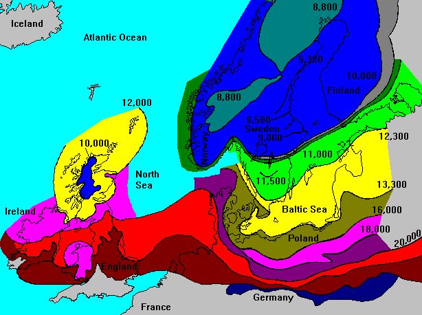
Map showing the extension of glaciers in Northern Europe and the phases of the Weichsel glaciers' withdrawal. The dark blue at the bottom in Germany represents the extent of the Elster Glaciation. Brown and Red represent the extent of the Saale glaciers. The other colors represent different stages of the Weichsel glacier's withdrawal. Here it is assumed that the Weichsel ice age had its maximum 20,000 years ago and that the edge of the glacier stood south of the Swedish lakes and along Norway's coast 11,711 years ago when the ice age ended. At the beginning of the Early Stone Age's Maglemose period, the ice covered the Norwegian mountains and northern Scandinavia. Thus, it took more than 12,000 years for the ice to melt away from the Scandinavian peninsula, and there are still glaciers in the Norwegian Mountains, Iceland and Greenland this day. 10% of Earth's surface is still covered by the remaining glaciers.
In recent years there has been an indication of a relatively warm climate in
Younger Dryas in the area around the Irming Sea (which is the sea east of Greenland) - both in Greenland and in the seabed off the coast. Similar observations have been made north of Iceland. This is in stark contrast to the strong cooling that otherwise took place at lower latitudes in the area around the North Atlantic. Maybe it really was so that the fresh melt-water, which was produced in the Arctic during the general warming, weakened the Gulf Stream thereby providing a cold spell in the areas further south. Also, it had been suggested that new prevailing winds created a more efficient exchange of heat and cold between the Arctic and the rest of the northern hemisphere.
A problem with the melting water pulse theory is that scientists have found signs of another melt-water pulse, a bit smaller than the first one, which occurred at the end of the Younger Dryas (Fairbanks, 1989). One may ask: why did this one not trigger another chain reaction in the climate system and a new cold spell?
|
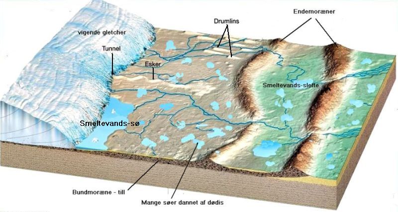
Landscape left by a receding glacier. The glaciers left a landscape with
thousands of lakes and streams. Under the glaciers, melt water flowed through
subglacial stream trenches, where they flowed out at the glacier edge, they formed deltas. Along the subglacial stream, trenches could be formed ridges, called eskers that emerged when the ice retreated. When the ice progressed over the existing landscape, it could polish existing landscape formations down to the elongated hills called drumlins. When the edge of the ice stood on the same place for a long time, were formed end moraines, which are longer elongated hills. All that soil and rock, which the ice dragged along and left
everywhere, are called ground moraine or "till" - to distinguish it from end moraines. All over small and large lakes were formed due to dead ice, which was chunks of ice that were covered with earth and stones, thereby isolated from the sun's heat and therefore preserved longer than the actual glacier. When the chunks finally melted they left holes, which were filled with water and thereby formed lakes. All that water and gravel, which flowed out from the melting glacier formed extensive water-rich meltwater plains. At the edge of the glacier were formed - often very large - ice lakes filled with ice-cold meltwater with floating icebergs.
In more recent times, some researchers have questioned the notion of glacier recession, as shown in this picture. They believe that the idea of the ice is such a massive wall that slowly retreated to the north is inspired by our knowledge of glaciers in mountains. They suggest that in a more flat terrain the ice would just become thinner and thinner and finally degenerate
to several distinct clumps of dead ice, which then created the thousands of lakes in the landscape after the Ice Age.
Towards the end of the Younger Dryas temperature in Greenland rose with no fewer than eight degrees in just 10 years, which is equivalent to that the climate of Scandinavia was replaced with a Mediterranean climate. One does not know what was the cause of this rapid change in temperature.
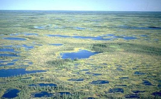
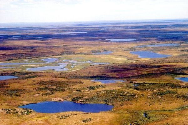
Landscape with many lakes in northern Canada. The melted glaciers left a water-rich landscape filled with big and small lakes, as we know from Canada and Finland. In northern Europe after the Ice Age were also left thousands of lakes, which in present time are often reduced to peat bogs.
The North American ice shield was larger than the Scandinavian and therefore took longer to melt; only 7,000 to 6,000 years ago the last inland ice disappeared from the area around Hudson Bay. The glaciers in the tropical parts of the Andes Mountains began to dwindle several thousand years before the warming in the northern hemisphere. The Inland ice in Greenland and Antarctica still exist and reminds us that we are living in an interglacial period, and one day the cold will come back.
The receding glaciers in northern Europe and North America left behind a water-rich landscape filled with thousands of lakes and small and large rivers, hills and hollows created by moraines and dead ice-holes and everywhere an abundance of stone and gravel, which the ice had dragged along.
On the thickest places, the ice could be up to three kilometers thick and lay there for thousands of years. Its huge weight pressed down the land. The depression was strongest where there was most ice, and in these places, land uplift is also greatest today.
|
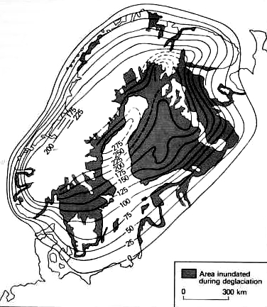
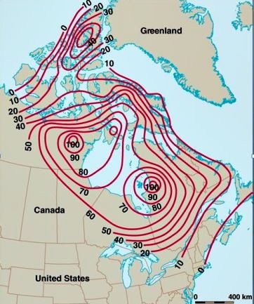
Left: Land uplift in Scandinavia since the end of the Weichsel ice age. The ice sheet over the Gulf of Bothnia was about three kilometers thick and lay there for many thousands of years, therefore, the country was depressed by the weight of the ice. Since the Ice Age ended, the land has slowly risen. In the area of the Gulf of Bothnia, the land since the Ice Age has lifted by up to 280 meters. Immediately after the disappearance of the ice the land was still depressed and was initially flooded; these areas are shown with darker color. Land uplift in Scandinavia is still taking place at a rate of up to 9 mm. per year around the Gulf of Bothnia.
Right: Land uplift in North America, since the Ice Age ended. Since the last ice melted away about 6,000 years ago, the country West and East of Hudson
Bay has lifted respectively 100 and 190 m, it is not as much as the
Scandinavian uplift, but in North America it is a shorter time ago that the ice loosened its grip. Land uplift is still taking place at a rate of 6 mm. per year in the area around Hudson Bay.
When the Weichsel ice age ended, the pressure relieved, and slowly the land began to rise, a process that is still ongoing to this day. Thus the area
around the Gulf of Bothnia is still lifting about 9 mm. per year and the area around Hudson Bay rises 6 mm. per year. Some Danish researchers believe that the expected future uplift in Scandinavia will more than match a feared increase in sea surface level due to the generally expected global warming.
As the ice retreated or simply degenerated on the spot and melted away, it left a landscape filled with thousands of small and large lakes. This happened because large chunks of preserved ice, so-called dead ice, gradually became
covered by gravel and stone supplied by the constant flow of melt-water, which
was produced by the continuous melting. Thereby, the dead ice-clumps became isolated against the sun's heat and melted many years later, leaving holes in the landscape, which became lakes. The typical landscape that emerged after the Weichsel Ice Age, must have resembled the landscape of Finland, northern Canada and Siberia, filled with lakes of all sizes.
|
Top: Arctic landscape full of lakes on Tamyr peninsula in northern
Siberia.
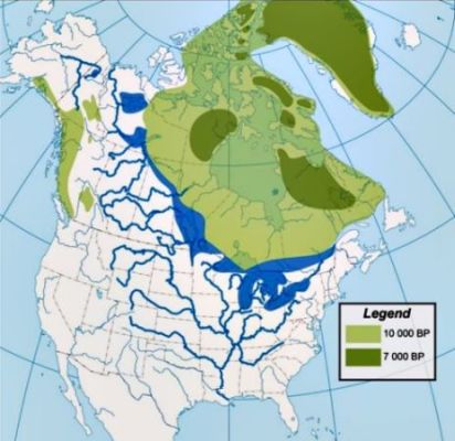
Bottom: Melt-water lakes along the margin of the North American Laurentide
Glacier about 10,000 years before present. It is seen that almost all the large lakes in North America have been created by melting of the last Ice Age's glaciers. (Denton and Hughes).
Not all melt-water ran directly into the sea through the rivers. The receding
inland ice created or exploited in many places depressions at the edge of the glaciers, which was filled with ice-cold water with melting floating icebergs.
The Great Lakes of North America between Canada and the United States, that is Lake Superior, Michigan, Huron, Eire, the St. Lawrence waterway and the great Canadian lakes, that is Lake Winnipeg, Great Slave Lake and Great Bear Lake and many others originated as such large glacial lakes at the edge of the ice sheet at the end of Pleistocene.

|
The freshwater lake called the Baltic Ice Lake was formed when the kilometers-thick Scandinavian ice sheet began to melt. It was a cold sea with floating icebergs. The lake surface was above World's sea surface level. Some believe that ice lake emptied by a major flood disaster around 9.600 BC, but most believe that it happened gradually.
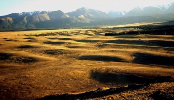
The landscape of northern Europe was dominated by mammoth steppe and regular tundra roamed by a small number of reindeer hunters.
After it had got a connection with the World Sea, it became a brackish sea, as we know it today. The Yoldia Sea owes its name to the mussel Yoldia Arctica. It was connected with the World Sea through a sound that was located where the Swedish lakes and the Gøta river are today.
The Maglemose hunters of the Stone Age could enjoy an increasingly warmer climate. At the beginning of their period, the tundra recently had been overgrown by an open and light birch forest mixed with aspen, willow, mountain ash and pine.
As Scandinavia was freed from the weight of ice masses, the land raised and the uplift cut off the coming Baltic Sea's connection with the World Sea, and
it became once again a freshwater lake called Ancylus Lake after the freshwater snail Ancylus fluviatilis. The Ancylus Lake had maybe drainage through the Great Lakes in Mid Sweden.
In step with the ever milder climate, where summer average temperature rose to 18-20 degrees, and winter temperatures barely passed below freezing, also the composition of the forest changed; pine pushed birch back and hazel, elm, oak, ash, alder, fir and linden immigrated.
At the end of the Maglemose hunters period, around 7,200 BC, the climate in Western Europe changed to the so-called Atlantic climate. It was a mild and humid coastal climate with summer temperatures 2-3 degrees higher than today. The sea surface level in the World Seas rose, which after some time caused the salty seawater to enter the Ancylus Lake, and the water in the Baltic Sea again became salty. The new sea is called Littorina Sea after the saltwater
snail Littorina littorea. It lasted several hundred years before the salt content reached its maximum.
Plants like mistletoe and the subtropical water-plant Trapa natans and animals like Dalmatian pelican and pond turtle became common in northern Europe. The land became covered by an impenetrable primeval forest.
The melting of the Scandinavian inland ice created the Baltic Ice Lake, which
was the beginning of the Baltic Sea. It later became a saltwater sea with a connection to the World Sea, but about 5,000 years before present, the World Ocean's access to the Baltic Sea had become so narrow that the salt content was reduced and the Baltic Sea became a brackish sea like the sea that we know today.
|
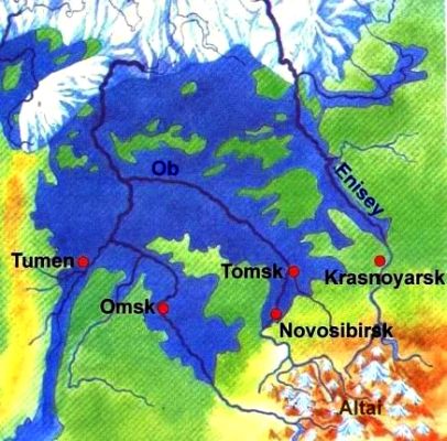
Top: Late-Pleistocene lake in the Western Siberian lowlands.
Bottom: Reconstruction of drainage in central Eurasia in late Pleistocene.
The big Swedish and Finnish lakes were all created by the melting inland ice,
as they were originally parts of both the Yoldia Sea and the fresh Ancylus Sea. Also the Russian Onega lake in Karelia and Peipus lake between Russia and Estonia - just to mention some of the largest - were created by the dwindling Weichel inland ice.
It has been found with certainty that one or more times during the Pleistocene a very large lake had existed in the area of the West Siberian lowlands, which are drained by the rivers Ob and Yenisei; the altitude of the lowlands seldoms exceeds 150 meters. Many carbon-14 tests from both river valleys have
confirmed that the lake last time existed between 22,000 and 12,300 before present. (Arkhipov 1973). One must assume that the lake's existence was due to that Obs and Jenisejs outlet in the Arctic Ocean at this time must have been blocked, probably by ice.
However, glaciers are formed by abundant precipitation in the form of snow, and it is surprising that glaciers in the Polar Sea could be formed so far away from the Gulf Stream's humidity and precipitation. In addition, the sea level at that time was quite low, so there must have been a pretty solid barrier.
|
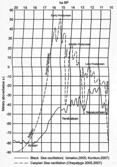
Top: Sea surface level in the Black Sea and the Caspian Sea during the late Pleistocene. Note that the Caspian Sea has been very water-rich precisely in
the Bølling-Allerød warm period, where one can expect that much melt-water was created. Furthermore, the graph of the water level in the Caspian Sea shows a marked fall that precisely coincides with the short cold spell between the Bølling and Allerød periods. This suggests that the high sea surface levels really were created by an inflow of melt-water from the north. By comparison with the diagram above showing the world the sea surface level, we see that the Black Sea almost all time had higher sea surface level, which indicates that it has been cut off from the world oceans. Only about 10,000 years before present, the World Sea, Black Sea and the Caspian Sea all have the same surface level, indicating that they all may have been connected vessels - Mechnikov National University Ukraine.
Bottom: Sea surface level variation in the Earth's oceans in the late Pleistocene and Holocene.From Wikipedia
The precise extent of such a large lake or lake system in western Siberia
has not yet been mapped. It is likely that it was also supplied with water from
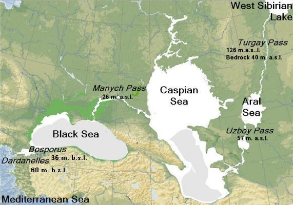
The Ob's and Jenisej's outspring in the mountains of central Siberia. The lake may have had drainage northward into the Arctic Ocean around an ice barrier or may have had drainage to the south. Based on existing topography of the area and the reconstructed depth of the lake, scientists have found it likely that it had drainage south to the Aral Sea and the Caspian Sea perhaps through the Turgay valley.
The existence of such a large West Siberian lake also indicates that Lake Baikal may have had an drainage to the Mediterranean through the world's longest river. Yenisei springs from Baikal and had back then drainage to the great West Siberian lake. The lake had by all appearances drainage through the Turgay valley to the Aral Sea, which at this time may have had a connection to the Caspian and Black Sea and then maybe continued to the Mediterranean with a large waterfall. Such a river would have been more than 10,000 kilometers long.
In Central Asia and North America occurred during the melting of the inland ice in Late Pleistocene huge devastating floods caused by dam collapse by gigantic lakes dammed by parts of glaciers in mountain valleys. Floods that had such strength and size that they bring our thoughts on the Biblical Flood.
|
Left: The Biblical Flood.
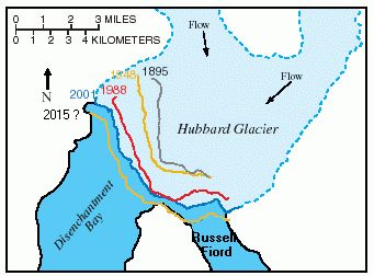
Right: Hubbard Glacier in Alaska - It is expected that after some years it
again will have expanded so much that it again will cut off Russell Fjord from
Disenchantment Bay and the sea. The surface level in Russel Fjord will again increase, and the ice dam will after some time again collapse.
The mechanism of the floods is illustrated quite good by the contemporary situation of Hubbard Glacier in Alaska.
The ice front of Hubbard glacier advanced through the centuries, and in May 1986 it pushed forward and blocked the outlet of Russell Fjord, creating "Russell Lake". All the summer's melt-water ran into in the new glacier-dammed lake and surface level increased by 25 meters.
Around midnight on 8. of October that year, the ice dam began to fail. In the
next 24 hours, a flood of estimated 5.3 km3 of water poured through the dam breach, and the fjord became reconnected to the sea. The flow rate corresponded to 35 times Niagara Falls.
Hubbard Glacier is still advancing, and it is foreseeable that it in a number of years again will cut off Russell Fjord, the water level in the new lake will again increase until the ice dam collapses, and a new flood will wash out into the sea.
Similar glacier-dammed lakes existed in late Pleistocene in the mountains of
southern Siberia and in the Rocky Mountains in North America - but on a much larger scale.
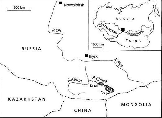
Kurai and Chuya were two late-Pleistocene glacier-dammed lakes in Altai mountains along the river Chuya.
The Russian geologist Alexei N. Rudoy has explored traces of giant floods
found in the Altai Mountains. He suggested the name diluvium for such changes in the landscape, which have been caused by catastrophic flood waves from
giant glacier-dammed lakes.
Towards the end of the last ice age, some think in the interval between 40
and 13 thousand years before present, glaciers in the Altai Mountains blocked the Chuya River, which is a tributary of the Katun, which in turn is a tributary of the Ob. Ice dams created at least two major glacial lakes of melt-water in the Chuya and Kurai valleys. After some time, the lakes became large and deep. Since ice is not a very resistant dam material, the dams busted in chain-reaction or each one separately, resulting in catastrophic floods that swept along Chuya and Katun rivers. In the time interval mentioned above, there were at least five major flooding.
Also in the Uymon valley in the Altai and the Darkhat Lakes in Mongolia existed glacier-dammed lakes in late Pleistocene.
Based on the estimated volume of the original glacier-dammed lakes, which have been rated to more than 600 km3, differences in altitude and cross-sections of the river valleys geologists have calculated some approximate water speeds to dozens of meters per second. Within a short time, that is a few days, clearly less than a week underwent the original landscapes enormous changes as a result of the late Pleistocene super-floods.
|
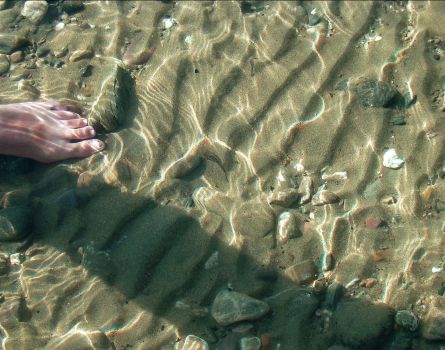
Left: Wave pattern on the bottom of a creek.
Right: Landscape with a gigantic wave pattern in the Altai Mountains, which testifies a gigantic flood wave in the past - photo by Alexei Rudoy July
2011.
In the sandy bottom of brooks and rivers is often seen a wave pattern formed by turbulent flow. Size and shape of the pattern depend on the velocity and volume of the flow. In Chuya and Katun valleys Rudoy and his colleagues found
areas with gigantic wave patterns, which indicate just as gigantic floods in the past. The wave landscape is made up of round pebbles, and the waves can
be up to 18 meters high having wavelengths of 50 to 150 meters.
Square river valleys along the Katun river in Altai, which testifies gigantic
devastating floods in the past - photo by Alexei Rudoy July 2011.
Rivers, which for millennia slowly have worked their way through the landscape, typically create V-shaped river valleys, such as the Rhine and Danube river valleys. Glaciers create typical U-shaped glacial valleys. But dynamic and devastating floods that are tearing its way through the land, create square valleys. In Altai, geologists found huge square river valleys, which testify gigantic devastating floods in the late Pleistocene.
Fast flowing rivers may form elongated banks of stone and gravel, which they have brought with them. They are called "gravel bars" in English. They are typically formed in the middle of the river or along one of the banks. In Altai Rudoy and his colleagues found very large "gravel bars", which in all probability have been deposited by huge fast flowing floods at the end of the ice age.
Such landscapes formed by huge floods once in the past have been found in several locations in Eurasia. In addition to the Altai Mountains, they have been found in both Tuva and Tibet.
|
Left: Common "Gravel bars" in the Toklat River in Alaska - photo QT Luong.
Right: Huge "Gravel bar" in central Altai, which testifies a huge volume flow, which took place in the past - photo by Alexei Rudoy July 2011.
Elizabeth Barber wrote in her book "The Mummies of Urumchi" that in the late Pleistocene Tarim Basin was a large lake. Chinese sources (Feng, Q., Z. Su, and H. Jin) write contrary: "The climate in the Tarim Basin has been persistently dry through alternating hot and cold periods. Consequently, the sedimentary environments have varied between desert and steppe strongly influenced by the surrounding mountains and the global climatic fluctuations." Other sources mention scattered forest combined with steppe. We must conclude that the climate in eastern central Asia through late Pleistocene probably have been a bit more fertile than today, but however relatively dry as precipitation in Central Asia has not been sufficient to form the same extensive glaciers, as in Scandinavia and North America.
|
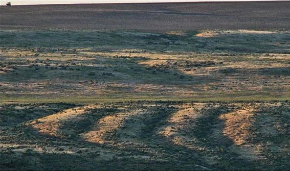
Top: Giant wave pattern at Washtucna Coulee
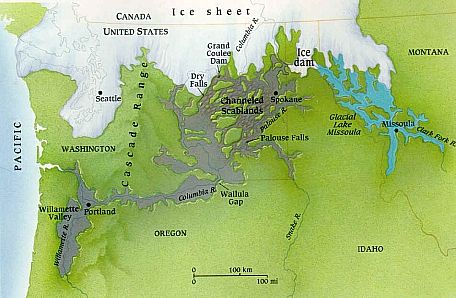
Bottom: The route of the Missoula flood waves and flooded areas through Montana, Idaho and Washington. Lake Missoula is shown in blue and the flooded areas, known as the Channeled Scablands, are shown in gray.
From North America are known two types of gigantic catastrophic floods namely the Missoula flood waves and the Bonneville flood wave. The Missoula flood waves came from the glacier-dammed Lake Missoula and occurred many times at
regular intervals. The Bonneville flood wave came from the moraine-dammed Lake Bonneville and occurred only once.
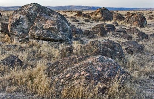
Large boulders that have been washed along with a Missoula flood wave.
Lake Missoula was a large glacier-dammed lake in western Montana, it existed in late Pleistocene during the period from 15,000 to 13,000 years before present. It was created by a glacier blocking of Clark Fork River. As with other glacier-dammed lakes, the ice dam collapsed at intervals, and the lake exhausted its water through the Clark Fork River's floodplain. Clark Fork River is a tributary of the Columbia River, which flows into the Pacific Ocean. The flood wave flooded large areas of the eastern state of Washington and the Willamette Valley in Western Oregon. Geologist J. Harlen Bretz proposed that the characteristic landscape in the state of Washington, which is called the Channeled Scablands, was created by repeated massive flooding through 2,000 years.
Judging from the coastlines, found in the valleys of Western Montana some have calculated that the Pleistocene Lake Missoula had a volume of about 2,200 km3.
Geologists estimate that the cycle of flooding and restoration of the lake took an average of 55 years. Jim O'Connor and Gerard Benito from the U.S. Geological Survey have found evidence of at least 25 massive flooding. The largest flood wave is believed to have had a volume flow of about 10 km3 per hour, which is 13 times the Amazon River flow.
|
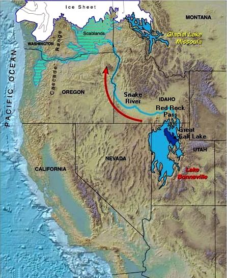
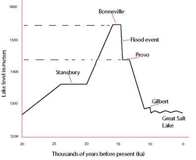
Left: Lake Bonneville in late Pleistocene 14,500 years before present. The
Pleistocene lakes are shown in light blue. The modern Great Salt Lake is shown in dark blue. The flood wave broke through at Red Rock Pass and spread northward into Idaho and Oregon along the Snake River until it reached Scablands in Washington, then it followed the route of the Missoula flood waves to the sea along Columbia river.
Right: The altitude of Lake Bonneville's shorelines in epochs of the lake's history - as explored by various geologists. The vertical scale on the left represents meters above the sea surface level. The horizontal scale shows years before present. It appears that the surface of Lake Bonneville was about 1,540 meters above sea surface level. After the flood, the lakes surface sunk to the Provo coastline around 100 meters lower. This means that a volume of 100 meters multiplied by the lake's area was flushed out into Idaho and Washington. Estimates of the lake area vary but if it was about 51,300 km2, it will make the volume of the flood wave to almost 5,130 km3.
Lake Bonneville was a very large lake in the state of Utah. The lake existed in late Pleistocene 14,500 years ago. The Great Salt Lake is the last remnant of the giant lake. Contrary to Lake Missoula, Lake Bonneville was a kind of moraine-dammed lake. The dam was created by gravel and stone that an Ice Age's glaciers had dragged along up and deposited on the lake's north end at Red Rock Pass in southeastern Idaho.
|
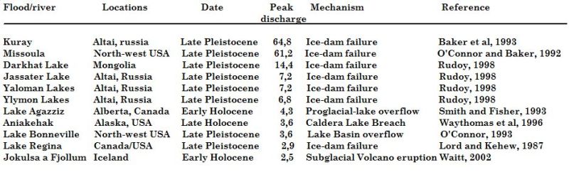
Large flood waves in the Quaternary following "The worlds largest floods, past and present: their causes and magnitudes" by Jim E. O'Connor and John E. Costa. However, volume flow under "Peak discharge" is here indicated in km3 per hour, as the author thinks it is a more descriptive unit.
Almost 15,000 years ago the barrier of rocks and gravel collapsed and Lake
Bonneville poured vast amounts of melt-water into the Red Rock Pass and beyond
into the Snake River Basin, where it caused widespread flooding. From there the flood continued along the Snake River in Idaho and Oregon until the
Columbia River Valley in Washington and then into the sea. One can imagine
that the breakthrough started as only a small trickle of water, which developed into a devastating flood wave that washed and tore everything along.
There's has been made many calculations on how fast the water flowed, but it is easy to imagine that with a vertical head of 100 m, it has been a very powerful flood.
|
Sea Level Versus Temperature af L. David Roper. (pdf) Ice Ages (Milankovitch Theory) af M. F. Loutre, Universite´ catholique de Louvain. - inkluderet graf, som viser Bergers kalkulation af Milankovitch insolation. (pdf) Statsgeolog beroliger: Danmark hæver sig mere end havet af Birgitte Marfelt i Ingeniøren. A giant Sirbirian Lake during the last Glacial: Evidence and Implications af E.U. Lioubimtseva, S.P. Gorshkov og J.M. Adams. Late Pleistocene and Holocene climate of SE Australia reconstructed from dust and river loads deposited offshore the River Murray Mouth. af Franz Gingele, Patrick De Deckker og Marc Norman. - Science Direct. (pdf) Earth's Climate History (Kindle Edition) by Anton Uriarte. |
| To start |